• Introduction

    In this project, I decided to discover patterns in the housing prices of California. Using a dataset of the housing prices in California’s districts, I aimed to use clustering to identify if there were any separating features within the dataset. I used k-means clustering to group the districts based on their population, prices, and house descriptions.

    Clustering

    K-means clustering is a method of clustering that uses quantitative data to identify patterns by creating groups of similar data-points. The model creates k amount of clusters based on the value of your choosing. After choosing your number of clusters, the model establishes centroids that act as the center of the clusters. The model then goes through your data and assigns each point to its most similar centroid. The model repeats this process until the data points stop moving.

    The Dataset

    https://www.kaggle.com/datasets/camnugent/california-housing-prices

    This Kaggle dataset contains information about housing districts within California. The features include the median house age, the total amount of rooms, the total amount of bedrooms, the population, the total number of households, the median income, the median house value, and location information.

    Data Understanding

    To check for collinearities, I created a correlation matrix of the dataset’s features. The matrix showed that features such as total rooms, households, and population all had high correlations, but I decided that these features had information that couldn’t be dropped. The matrix also showed that the locational information, such as longitude and latitude, had high correlation with one another. I decided to drop these features because I felt the location of the district would interfere with any insights. If we were to group the districts with location, the districts would just be placed into clusters based on their physical distance from each other.

    Data Preprocessing and Modeling

    First, I dropped the longitude, latitude, and ocean proximity from the dataset. I did this to remove the physical distance of the districts from being a factor, and because ocean proximity was not a quantitative feature. Next, I found the average amount of rooms and bedrooms of each district by dividing the total amount of rooms and bedrooms by the total amount of households and added them to the dataset. I did this so that the dataset would have more information on individual houses within the district. Then, I normalized the dataset so that outlying districts wouldn’t affect the model negatively. Afterwards, I checked the data for any null values and dropped the bedroom features because they had null values. I dropped these features instead of replacing the null values because I felt that the room features gave enough information about the rooms within a house. Finally, I applied PCA to summarize the features, and to make the modeling more efficient. To choose the number of components for PCA, I plotted the explained variance against the number of components. This led me towards choosing 2 components for PCA because it was the lowest amount of components with a sufficient amount of explained variance. After the preprocessing, I ran the k-means model with different amounts of clusters and used the elbow method to choose k. I also used the different amounts’ silhouette score to make sure I choose a sufficient k. Using the elbow method and silhouette scores, I chose 2 clusters for the model.

    Model Insights

    Once the model assigned each district its cluster, I created boxplots for each of the features separated by the clusters. The boxplots showed that the first cluster had districts with older houses, as well as districts with lower populations and households. Conversely, the second cluster had newer houses and a higher population with more households. There were very slight differences between each cluster’s income and house value.

    Impact

    Using this model, we could easily identify the housing needs of each district within California. Districts that fall within the first cluster could be classified as districts that need housing built. Building more houses within these districts could result in the population of each district being distributed more evenly, but this model fails to determine whether this is actually plausible. Theses districts could have conditions that restrict the building of houses, and this model is unable to determine those conditions. The upside to this model is that it allows us to narrow down the amount of districts that need new housing.

    Code

    https://github.com/cpham10-charlotte/itcs3162_project4

    Introduction

    This project uses a dataset of measurements and information about crocodiles to predict the habitat and conservation status of a given crocodile. The aim of the project was to use the length and width of a crocodile to predict its habitat, but also use the length, width, and habitat to predict its conservation status.

    Introducing the Data

    The dataset I used in this project is a collection of observed information about species of crocodiles. I found this data set on Kaggle (https://www.kaggle.com/code/gpreda/crocodiles-species-around-the-world). The dataset contains the crocodile’s common name and scientific name, the observed weight and length, the age class, the sex, the date of observation, the country and habitat, and the conservation status of the crocodile. In the dataset, the age class was broken up into “Hatchling”, “Juvenile”, “Subadult”, and “Adult”.

    Pre-Processing the Data

    When going into this data, I decided that only the measurements, habitat, and conservation status were useable for classification. So, when I split the data into just the measurements, and I used the habitat and conservation status as targets. The measurements and habitat didn’t need any cleaning up aside from being separated from the dataset. The conservation status had entries that were considered “Data Deficient”, so I removed the “Data Deficient” entries when I was using the conservation status as the targets. For all of this data to make sense, I limited the data I used to the recorded data for crocodiles in the “Adult” class. I only used the “Adult” class because I didn’t know the growth rates of each crocodile, and the “Adult” age class had the most entries among the age classes.

    The Model

    The model I chose for this problem is the k-NN model. The k-NN model classifies the given data by distance. The model chooses k neighbors for each point and classifies the point by its nearest neighbors. K-NN applies no weight to each feature, which is a pro and con depending on the situation, it requires no prior assumptions for its classification, and its incredibly simple. The cons of k-NN are that its computationally costing with extremely large datasets, and that the model does not perform well with high dimensionality. I chose this model because I imagined plotting the measurements would create areas that aligned with the targeted prediction, and the crocodile dataset wasn’t too large.. At first, I fit the model to predict the habitat of the crocodile using the measurements, but this model was incredibly inaccurate. I decided to change my target to the conservation status, and I moved the habitat into the model data as a result. Now the data included the observed measurements and the habitat of a given crocodile, which was used to predict its conservation status. This resulted in a model with higher accuracy, but the model still had low accuracy in general. To evaluate the model’s accuracy, I used the accuracy score of the model. I used accuracy score because there are no incredible consequences for being accurate for the wrong reasons.

    The Story around the Data

    Coming into this project, I thought that the measurements from the data would create clusters, but the measurements plotted out pretty closely to a logarithmic curve. I didn’t think this would create any problems for my model, but I think this might have been the reason for my model’s poor performance. This might have improved had I used a different model, which is something I’ll keep in mind for the next project.

    Impact

    This project, had it gone successfully, could have predicted the danger of endangerment a crocodile species would face. This model could do major damage to those predicted false negative because it would cause attention to be taken away from the species that really needed it.

    Code

    https://github.com/cpham10-charlotte/itcs3162_project2

  • Introduction

    This project uses a dataset of measurements and information about crocodiles to predict the habitat and conservation status of a given crocodile. The aim of the project was to use the length and width of a crocodile to predict its habitat, but also use the length, width, and habitat to predict its conservation status.

    Introducing the Data

    The dataset I used in this project is a collection of observed information about species of crocodiles. I found this data set on Kaggle (https://www.kaggle.com/code/gpreda/crocodiles-species-around-the-world). The dataset contains the crocodile’s common name and scientific name, the observed weight and length, the age class, the sex, the date of observation, the country and habitat, and the conservation status of the crocodile. In the dataset, the age class was broken up into “Hatchling”, “Juvenile”, “Subadult”, and “Adult”.

    Pre-Processing the Data

    When going into this data, I decided that only the measurements, habitat, and conservation status were useable for classification. So, when I split the data into just the measurements, and I used the habitat and conservation status as targets. The measurements and habitat didn’t need any cleaning up aside from being separated from the dataset. The conservation status had entries that were considered “Data Deficient”, so I removed the “Data Deficient” entries when I was using the conservation status as the targets. For all of this data to make sense, I limited the data I used to the recorded data for crocodiles in the “Adult” class. I only used the “Adult” class because I didn’t know the growth rates of each crocodile, and the “Adult” age class had the most entries among the age classes.

    The Model

    The model I chose for this problem is the k-NN model. The k-NN model classifies the given data by distance. The model chooses k neighbors for each point and classifies the point by its nearest neighbors. K-NN applies no weight to each feature, which is a pro and con depending on the situation, it requires no prior assumptions for its classification, and its incredibly simple. The cons of k-NN are that its computationally costing with extremely large datasets, and that the model does not perform well with high dimensionality. I chose this model because I imagined plotting the measurements would create areas that aligned with the targeted prediction, and the crocodile dataset wasn’t too large.. At first, I fit the model to predict the habitat of the crocodile using the measurements, but this model was incredibly inaccurate. I decided to change my target to the conservation status, and I moved the habitat into the model data as a result. Now the data included the observed measurements and the habitat of a given crocodile, which was used to predict its conservation status. This resulted in a model with higher accuracy, but the model still had low accuracy in general. To evaluate the model’s accuracy, I used the accuracy score of the model. I used accuracy score because there are no incredible consequences for being accurate for the wrong reasons.

    The Story around the Data

    Coming into this project, I thought that the measurements from the data would create clusters, but the measurements plotted out pretty closely to a logarithmic curve. I didn’t think this would create any problems for my model, but I think this might have been the reason for my model’s poor performance. This might have improved had I used a different model, which is something I’ll keep in mind for the next project.

    Impact

    This project, had it gone successfully, could have predicted the danger of endangerment a crocodile species would face. This model could do major damage to those predicted false negative because it would cause attention to be taken away from the species that really needed it.

    Code

    https://github.com/cpham10-charlotte/itcs3162_project2

  • Introducing the Problem

    The data set I chose to look at is Hudl Statsbomb’s free release of their match record for the 2020 UEFA Euros. The “problem” that I chose to tackle with this data is to discover the key players for the top teams in the tournament. The definition of key player I chose are players with the most utilization within the tournament, and the top teams that I would look at are the teams that sat at the top of the FIFA rankings at the time. This definition of key player would mean that I would look to find the players with the most minutes played, the most passes, the most carries, etc.

    Introducing the Data

    Hudl Statsbomb’s 2020 UEFA Euros dataset is accessible through a free python library, and it has statistics for all of the matches played in the tournament. These statistics include, but are not limited to, blocks, tackles, carries, passes, shots, xG, and location data for applicable events. These statistics are separated into distinct events within each match.

    Data Pre-Processing

    When pre-processing the data, I used my pre-existing knowledge of soccer to understand, for the most part, what statistics I was looking for. With my goal to look for the most utilized players, I decided that I would look for the players that had the ball the most, and to determine who had the ball the most, I looked for the players that carried the ball and passed the ball the most. To do so, I filtered the data for events that were considered carries and stored that within a variable, and then did the same for events that were considered passes. I then separated the data so that these stats were only compared against directly against players within the same team.

    Visualizations

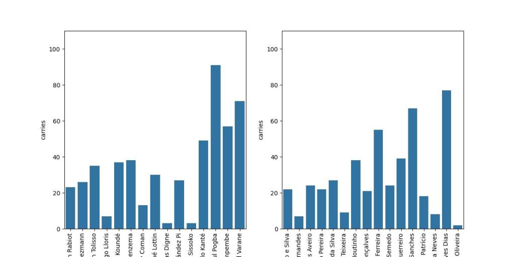
    Carries for Portugal vs France

    In this visualization, we can see that Paul Pogba, Raphael Varane, Presnel Kimpembe, and N’golo Kante have the most carries for France. For Portugal, Ruben Dias, Renato Sanches, Pepe (Kepler Ferreira), and Raphael Guerreiro have the most carries.

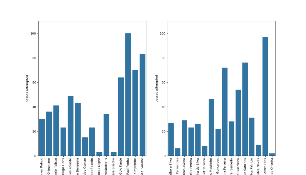
    Passes for Portugal vs France

    In this visualization, Paul Pogba, Raphael Varane, Presnel Kimpembe, and N’golo Kante have the most passes attempted for France. For Portugal, Ruben Dias, Renato Sanches, Pepe, and Raphael Guerreiro have the most passes attempted.

    For both teams, their midfielders and center-backs have the most carries and passes. This observations allows us to infer that both teams tend to play out of the back half of the field. To provide more detail, this means that Portugal and France aim to use the midfielders and center-backs to hold possession of the ball and progress the ball up the field.

    Impact

    The definition of a key player for any team varies widely between different people. This means that the stats that I used within this visualizations might not help determine who was vital to these top teams for other people. Another limitation of these visualizations is that they only include data from when Portugal and France played each other. With more data from other matches, these stats could change drastically, which would make these observations obsolete.

    Summary

    Using my definition of key player, I determined that for both France and Portugal, the back half of their teams were key for their success in the tournament. Both teams asked their defenders and midfielders to have the ball for most of the match.

    References

    https://www.hudl.com/blog/hudl-statsbomb-free-euro-2025-data

    https://www.hudl.com/blog/using-hudl-statsbomb-free-data-in-python

    https://github.com/statsbomb/statsbombpy

    Code

    https://github.com/cpham10-charlotte/itcs3162_project1

    Introduction

    This project uses a dataset of measurements and information about crocodiles to predict the habitat and conservation status of a given crocodile. The aim of the project was to use the length and width of a crocodile to predict its habitat, but also use the length, width, and habitat to predict its conservation status.

    Introducing the Data

    The dataset I used in this project is a collection of observed information about species of crocodiles. I found this data set on Kaggle (https://www.kaggle.com/code/gpreda/crocodiles-species-around-the-world). The dataset contains the crocodile’s common name and scientific name, the observed weight and length, the age class, the sex, the date of observation, the country and habitat, and the conservation status of the crocodile. In the dataset, the age class was broken up into “Hatchling”, “Juvenile”, “Subadult”, and “Adult”.

    Pre-Processing the Data

    When going into this data, I decided that only the measurements, habitat, and conservation status were useable for classification. So, when I split the data into just the measurements, and I used the habitat and conservation status as targets. The measurements and habitat didn’t need any cleaning up aside from being separated from the dataset. The conservation status had entries that were considered “Data Deficient”, so I removed the “Data Deficient” entries when I was using the conservation status as the targets. For all of this data to make sense, I limited the data I used to the recorded data for crocodiles in the “Adult” class. I only used the “Adult” class because I didn’t know the growth rates of each crocodile, and the “Adult” age class had the most entries among the age classes.

    The Model

    The model I chose for this problem is the k-NN model. The k-NN model classifies the given data by distance. The model chooses k neighbors for each point and classifies the point by its nearest neighbors. K-NN applies no weight to each feature, which is a pro and con depending on the situation, it requires no prior assumptions for its classification, and its incredibly simple. The cons of k-NN are that its computationally costing with extremely large datasets, and that the model does not perform well with high dimensionality. I chose this model because I imagined plotting the measurements would create areas that aligned with the targeted prediction, and the crocodile dataset wasn’t too large.. At first, I fit the model to predict the habitat of the crocodile using the measurements, but this model was incredibly inaccurate. I decided to change my target to the conservation status, and I moved the habitat into the model data as a result. Now the data included the observed measurements and the habitat of a given crocodile, which was used to predict its conservation status. This resulted in a model with higher accuracy, but the model still had low accuracy in general. To evaluate the model’s accuracy, I used the accuracy score of the model. I used accuracy score because there are no incredible consequences for being accurate for the wrong reasons.

    The Story around the Data

    Coming into this project, I thought that the measurements from the data would create clusters, but the measurements plotted out pretty closely to a logarithmic curve. I didn’t think this would create any problems for my model, but I think this might have been the reason for my model’s poor performance. This might have improved had I used a different model, which is something I’ll keep in mind for the next project.

    Impact

    This project, had it gone successfully, could have predicted the danger of endangerment a crocodile species would face. This model could do major damage to those predicted false negative because it would cause attention to be taken away from the species that really needed it.

    Code

    https://github.com/cpham10-charlotte/itcs3162_project2

  • Welcome to WordPress! This is your first post. Edit or delete it to take the first step in your blogging journey.

    Introduction

    This project uses a dataset of measurements and information about crocodiles to predict the habitat and conservation status of a given crocodile. The aim of the project was to use the length and width of a crocodile to predict its habitat, but also use the length, width, and habitat to predict its conservation status.

    Introducing the Data

    The dataset I used in this project is a collection of observed information about species of crocodiles. I found this data set on Kaggle (https://www.kaggle.com/code/gpreda/crocodiles-species-around-the-world). The dataset contains the crocodile’s common name and scientific name, the observed weight and length, the age class, the sex, the date of observation, the country and habitat, and the conservation status of the crocodile. In the dataset, the age class was broken up into “Hatchling”, “Juvenile”, “Subadult”, and “Adult”.

    Pre-Processing the Data

    When going into this data, I decided that only the measurements, habitat, and conservation status were useable for classification. So, when I split the data into just the measurements, and I used the habitat and conservation status as targets. The measurements and habitat didn’t need any cleaning up aside from being separated from the dataset. The conservation status had entries that were considered “Data Deficient”, so I removed the “Data Deficient” entries when I was using the conservation status as the targets. For all of this data to make sense, I limited the data I used to the recorded data for crocodiles in the “Adult” class. I only used the “Adult” class because I didn’t know the growth rates of each crocodile, and the “Adult” age class had the most entries among the age classes.

    The Model

    The model I chose for this problem is the k-NN model. The k-NN model classifies the given data by distance. The model chooses k neighbors for each point and classifies the point by its nearest neighbors. K-NN applies no weight to each feature, which is a pro and con depending on the situation, it requires no prior assumptions for its classification, and its incredibly simple. The cons of k-NN are that its computationally costing with extremely large datasets, and that the model does not perform well with high dimensionality. I chose this model because I imagined plotting the measurements would create areas that aligned with the targeted prediction, and the crocodile dataset wasn’t too large.. At first, I fit the model to predict the habitat of the crocodile using the measurements, but this model was incredibly inaccurate. I decided to change my target to the conservation status, and I moved the habitat into the model data as a result. Now the data included the observed measurements and the habitat of a given crocodile, which was used to predict its conservation status. This resulted in a model with higher accuracy, but the model still had low accuracy in general. To evaluate the model’s accuracy, I used the accuracy score of the model. I used accuracy score because there are no incredible consequences for being accurate for the wrong reasons.

    The Story around the Data

    Coming into this project, I thought that the measurements from the data would create clusters, but the measurements plotted out pretty closely to a logarithmic curve. I didn’t think this would create any problems for my model, but I think this might have been the reason for my model’s poor performance. This might have improved had I used a different model, which is something I’ll keep in mind for the next project.

    Impact

    This project, had it gone successfully, could have predicted the danger of endangerment a crocodile species would face. This model could do major damage to those predicted false negative because it would cause attention to be taken away from the species that really needed it.

    Code

    https://github.com/cpham10-charlotte/itcs3162_project2